Topology optimization of a 3D cantilever beam using body-fitted meshes#
The goal of this tutorial is to run a topology optimization of a 3D cantilever beam using body-fitted meshes.
Note
For running this tutorial Code_Aster 2 needs to be installed and available from the command line.
Test case#
Consider the following specifications
domain of size \(2\) m \(\times 0.25\) m \(\times 1\) m
elastic material with Young modulus equal to \(210.e9\) Pa and Poisson ratio equal to \(0.3\)
beam clamped on the plane \(x = 0\) m and submitted to a vertical load g = \((0, 0, -10000)\) N on the point \((2, 0.25, 0.5)\)
minimization of the volume under a compliance constraint
Data setting : header#
At first, we start by editing a Cantilever.xml file.
The data file starts with the following header
<data dim="3">
Data setting : implicit zones#
Define implicit zones
<Zones>
    <Plane id="1" point="0.0001 0.25 0.5" normal="1. 0. 0." desc="x0 plane"/>
    <Plane id="2" point="0.05 0.25 0.5" normal="1. 0. 0." desc="dirichlet"/>
    <Plane id="3" point="1. 0.24999 0.5" normal="0. -1. 0." desc="symetry plane"/>
    <Sphere id="4" center="2. 0.25 0.5"  radius="0.0009" desc="nodal force"/>
    <Cylinder id="5" center1="1.9999 0.25 0.5" center2="2.1 0.25 0.5" radius="0.01" desc="force"/>
    <Cylinder id="6" center1="-0.1 0.25 0.5" center2="2.1 0.25 0.5" radius="0.249"/>
    <Union id="7" z="2 4 6" desc="initialization"/>
    <Union id="8" z="2 5" desc="onzone"/>
</Zones>
Data setting : grids#
Define the background mesh which is a uniform grid
<Grids>
    <Grid id="1" n="41 41 41" origin="0. 0. 0." length="2.0 0.25 1.0" ofTetras ="True"/>
</Grids>
Data setting : levelsets#
Define the level set together with a set of options. The option conform=”True” means that the level set is conformal. When the body-fitted option is activated a set of meshing options are defined to drive the remeshing process.
<LevelSets>
    <LevelSet id="1" support="1" conform="True" gradientMethod="gradPhi">
        <MesherInfo hmax=".5" hmin="0.01" iso="0.0" rmc="1e-5"
        nr="True" computeDistanceWith="meshdist"/>
    </LevelSet>
</LevelSets>
Data setting : physical problems#
Define the physical problem, which is a linear elastic static problem.
We define material properties, two dirichlet conditions -clamped part and symetry plane- and one neumann condition.
By default we use linear elements.
<PhysicalProblems>
     <GeneralAster type="static_elastic" id="1" >
               <Material  young="210.e9" poisson="0.3" />
               <Dirichlet eTag="eTag1" dofs="0 1 2" value="0.0"/>
               <Dirichlet eTag="eTag3" dofs="1" value="0.0"/>
               <Force nTag="nTag4" value="0. 0. -10000" />
      </GeneralAster>
 </PhysicalProblems>
Data setting : outputs#
Define the desired output
<Outputs>
   <Output id="2" name="Cantilever.xdmf"/>
   <Output id="3" name="Cantilever.csv" nTag="nTag4" />
   <Output id="1" name="PROXY" outputs="2 3"/>
</Outputs>
Data setting : optimization problems#
Then, we define the optimization problem by entering the objective, the constraints, the initial levelset, the implicit zones, the output and a set of options.
Note that we have to define an upper bound value for the constraint.
Note that, since the constraint is a physical criterion, we precise which physical problem should be used with the keyword useProblem=”1”.
<OptimProblems>
    <OptimProblem type="TopoGeneric" id="1"
        OnZone="8"
        useLevelset="1"
    printMeshQualityInfo = "True"
        output="3"
        outputEveryLevelsetUpdate = "False">
      <Objective  type="Volume"  name="Volume"/>
      <Constraint type="Compliance"  name="Compliance" UpperBound="2.5*4.69434000e-01"   useProblem="1" />
   </OptimProblem>
</OptimProblems>
Data setting : optimization algorithms#
Then, we define the optimization algorithm which is linked to the optimization problem
<TopologicalOptimizations>
    <OptimAlgoNullSpace id="1"
       useOptimProblem="1"/>
</TopologicalOptimizations>
Actions setting#
Here we declare actions which must be runned. At first the level set “1” is initialized with the implicit zone “7”
<Actions>
    <Action type="InitLevelset" ls="1" zone="7"/>
Then, we add the bounding box edges and the skin to the initial grid. Moreover, we create tags on elements of dimension 2 starting from the implicit zones “1”,”3”. Tags “eTag1”,”eTag3” are created.
<Action type="AddEdges" ls="1" ar="90+45" />
<Action type="AddSkin" ls="1"/>
<Action type="CreateTagsFromZones" ls="1" elementTags="1 3" dim="2" elemenprefix="eTag"/>
We create a nodal tag “nTag4” from implicit zone “4” for the nodal force and we set it as required to preserve it during the remeshing
<Action type="CreateTagsFromZones" ls="1" nodalTags="4" nodalprefix="nTag"/>
<Action type= "SetAsRequired" ls="1" nTags="nTag4" />
We perform a remeshing to generate a conformal mesh
  <Action type="Remesh" ls="1" hmax=".5" hmin="0.01" iso="0.0" rmc="1e-5"
nr="True" computeDistanceWith="meshdist" />
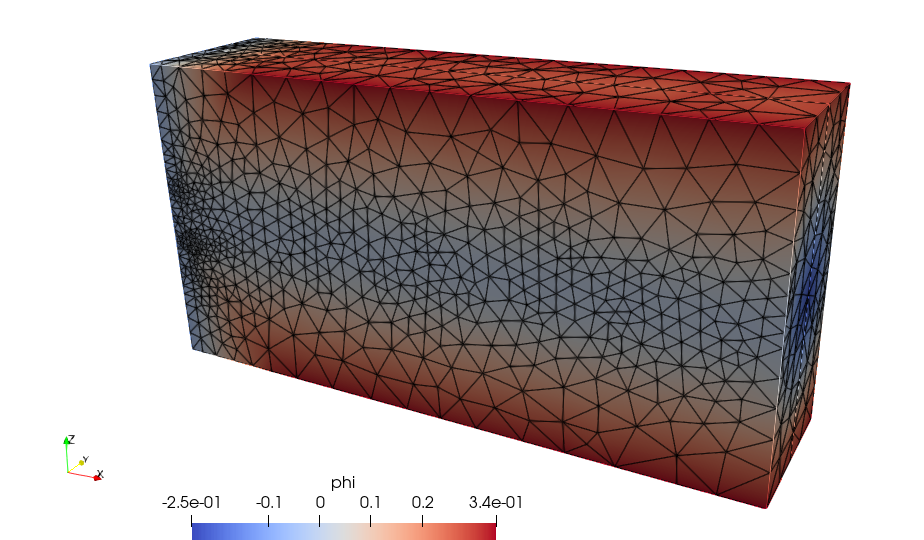
Fig. 7 Background mesh after a first remeshing#

Fig. 8 Cut of the initial body-fitted mesh#
Then, we run the topology optimization
<Action type="RunTopoOp" TopoOp="1"/>
Eventually the optimal shape is exported in stl format
       <Action type="SaveShapeToFile" ls="1" filename="Cantilever.stl"/>
   </Actions>
</data>
Run#
To run the script using the command line application execute in a terminal
OpenPiscoCL Cantilever.xml
To run the script using the GUI application execute in a terminal
OpenPisco Cantilever.xml
Output#
After running the tutorial script the following output files have been created in the working directory
Cantilever.xml.log : run summary
Cantilever.stl : optimal shape in stl format
Cantilever.xdmf : (heavy) file containing the mesh and fields at each iteration in xdmf format
Cantilever.csv : convergence history in csv format
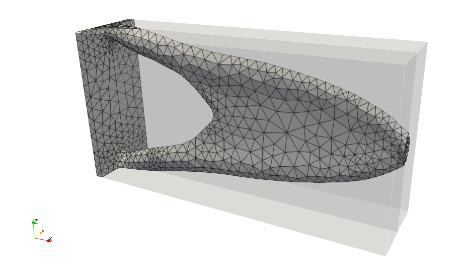
Fig. 9 Visualisation of the optimal design in Paraview#
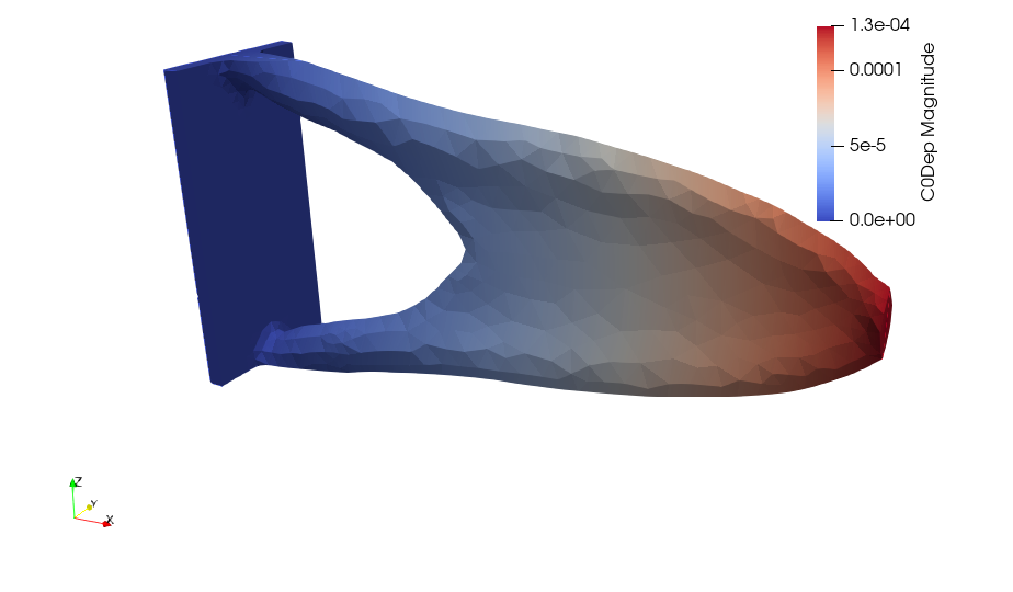
Fig. 10 Visualisation of the displacement field in Paraview#
The demo xml file created is available in the module OpenPisco.Demos() of the OpenPisco Python library 1 .