Topology optimization of a 2D bridge using body-fitted meshes#
The goal of this tutorial is to run a topology optimization using solely the OpenPisco Python library.
Test case#
Consider the following specifications
domain of size \(8\) m \(\times 2\) m
elastic material with Young modulus equal to \(1\) Pa and Poisson ratio equal to \(0.3\)
beam clamped on two regions on the plane \(y=0\) and submitted to a vertical load g = \((0, -0.002)\) N on the plane \(y=2\)
minimization of the compliance under a volume constraint
Data setting : imports#
We start by editing a Bridge.py file and importing all the needed modules
import numpy as np

from Muscat.MeshTools.MeshCreationTools import CreateSquare
from Muscat.ImplicitGeometry.ImplicitGeometryObjects import CreateImplicitGeometryPlane, ImplicitGeometryHoles,CreateImplicitGeometryAnalytical
from Muscat.ImplicitGeometry.ImplicitGeometryOperators import ImplicitGeometryUnion, ImplicitGeometryIntersection
from Muscat.MeshContainers.Filters.FilterObjects import ElementFilter
from Muscat.IO.XdmfWriter import XdmfWriter

from OpenPisco.Unstructured.Levelset import LevelSet
from OpenPisco.PhysicalSolvers.UnstructuredFEAGenericSolver import CreateUnstructuredFEAGenericProblem
from OpenPisco.Optim.Problems.OptimProblemTopoGeneric import OptimProblemTopoGeneric
from OpenPisco.Optim.Criteria.GeoCriteria import TopoCriteriaVolume
from OpenPisco.Optim.Criteria.PhyCriteria import TopoCriteriaCompliance
from OpenPisco.Optim.Algorithms.OptimAlgoNullSpace import OptimAlgoNullSpace
Data setting : implicit zones#
Define implicit zones
IGHoles = ImplicitGeometryHoles()
IGHoles.r = 0.2
IGHoles.n = np.array([6., 4., 2.])
IGHoles.type = "Original"

IGGeometryPlane = CreateImplicitGeometryPlane({"point": [0, 1.8, 0], "normal": [0, -1, 0]})

IGAnalytical1 = CreateImplicitGeometryAnalytical({"expr": "x-1 "})
IGAnalytical2 = CreateImplicitGeometryAnalytical({"expr": "x-7 "})
IGAnalytical2.insideOut = True
IGAnalytical3 = CreateImplicitGeometryAnalytical({"expr": "y-0.01 "})

IGUnion = ImplicitGeometryUnion([IGAnalytical1,IGAnalytical2])
IGIntersection = ImplicitGeometryIntersection([IGUnion,IGAnalytical3])
Data setting : grids#
Define the initial background mesh which is a uniform grid
dimensions = np.array([25,20])
length = np.array([8,2])
mesh= CreateSquare(dimensions=dimensions, spacing=length/(dimensions-1), origin=[0,0], ofTriangles=True)
Add ridges and corners to the mesh
for _,data,_ in ElementFilter(dimensionality=1)(mesh):
    data.tags.CreateTag("Ridges",False).SetIds(np.arange(data.GetNumberOfElements()))

mesh.nodesTags.CreateTag("Corners",errorIfAlreadyCreated=False).Merge(other=mesh.nodesTags[ "x0y0"])
mesh.nodesTags.CreateTag("Corners",errorIfAlreadyCreated=False).Merge(other=mesh.nodesTags[ "x1y0"])
mesh.nodesTags.CreateTag("Corners",errorIfAlreadyCreated=False).Merge(other=mesh.nodesTags[ "x0y1" ])
mesh.nodesTags.CreateTag("Corners",errorIfAlreadyCreated=False).Merge(other=mesh.nodesTags[  "x1y1" ])
Create mesh tag on elements of dimensionality equal to 1 for Dirichlet boundary condition
ff = ElementFilter()
ff.SetZones([IGIntersection])
ff.SetDimensionality(1)
for _,data,ids in ff(mesh):
    data.tags.CreateTag("Dirichlet").SetIds(ids)
Print the mesh
print(mesh)
Data setting : levelsets#
Define the level set together with a set of options. A set of meshing options are defined to drive the remeshing process.
levelset = LevelSet(support=mesh)
levelset.conform = True
levelset.MesherInfo = {"gradientMethod":"gradPhi","hmax":0.1,"hmin":0.01,"rmc":1e-5,"hausd":0.01,"nr":True,"iso":0.0}

IGHoles.SetSupport(levelset.support)
levelset.phi = IGHoles(levelset.support)
Data setting : physical problems#
Define the physical problem, which is a linear elastic static problem.
We define material properties, one dirichlet condition and one neumann condition.
The linear solver used is Mumps 2.
material = ('Material', {'young': '1', 'poisson': '0.3'})
dirichlet = ('Dirichlet', {'eTag': 'Dirichlet', 'dofs': '0 1', 'value': '0'})
load = ('Force', {'eTag': 'Y1', 'dir': '0 1', 'value': '-0.002'})
data = {'type': 'static_elastic', 'p': '1','dimensionality':'2',"linearSolverName":"Mumps",'children':[material,dirichlet,load]}
physicalSolver = CreateUnstructuredFEAGenericProblem(data)
Data setting : optimization problems#
Then, we define the optimization problem by entering the objective, the constraints, the initial levelset, the fixed implicit zone and a set of options.
Note that we have to define an upper bound value for the constraint.
res = OptimProblemTopoGeneric()
volCrit = TopoCriteriaVolume()
comCrit = TopoCriteriaCompliance()
res.SetObjectiveCriterion(comCrit)
res.AddInequalityConstraint(volCrit)
volCrit.SetUpperBound(0.4*1.55651243e+01)
comCrit.problem = physicalSolver
res.point = levelset
res.ResetState()
res.OnZone = IGGeometryPlane
Data setting : outputs#
Define the writer to get the output files
writer = XdmfWriter('Bridge2DHistory.xmf')
print("Opening file :"+writer.fileName)
writer.SetTemporal()
writer.SetBinary()
writer.SetXmlSizeLimit(0)
writer.Open()
res.writer = writer
Data setting : optimization algorithms#
Then, we define the optimization algorithm which is linked to the optimization problem
OA = OptimAlgoNullSpace()
OA.ResetState()
OA.alphaC = 0.5
OA.tol_merit =  0.001
OA.optimProblem =res
Run#
Run the topology optimization
OA.Start()
To run the script execute in a terminal
python Bridge.py
Output#
After running the tutorial script the following output files have been created in the working directory
Bridge.xml.log : run summary
BridgeHistory.xmf : (heavy) file containing the mesh and fields at each iteration in xmf format
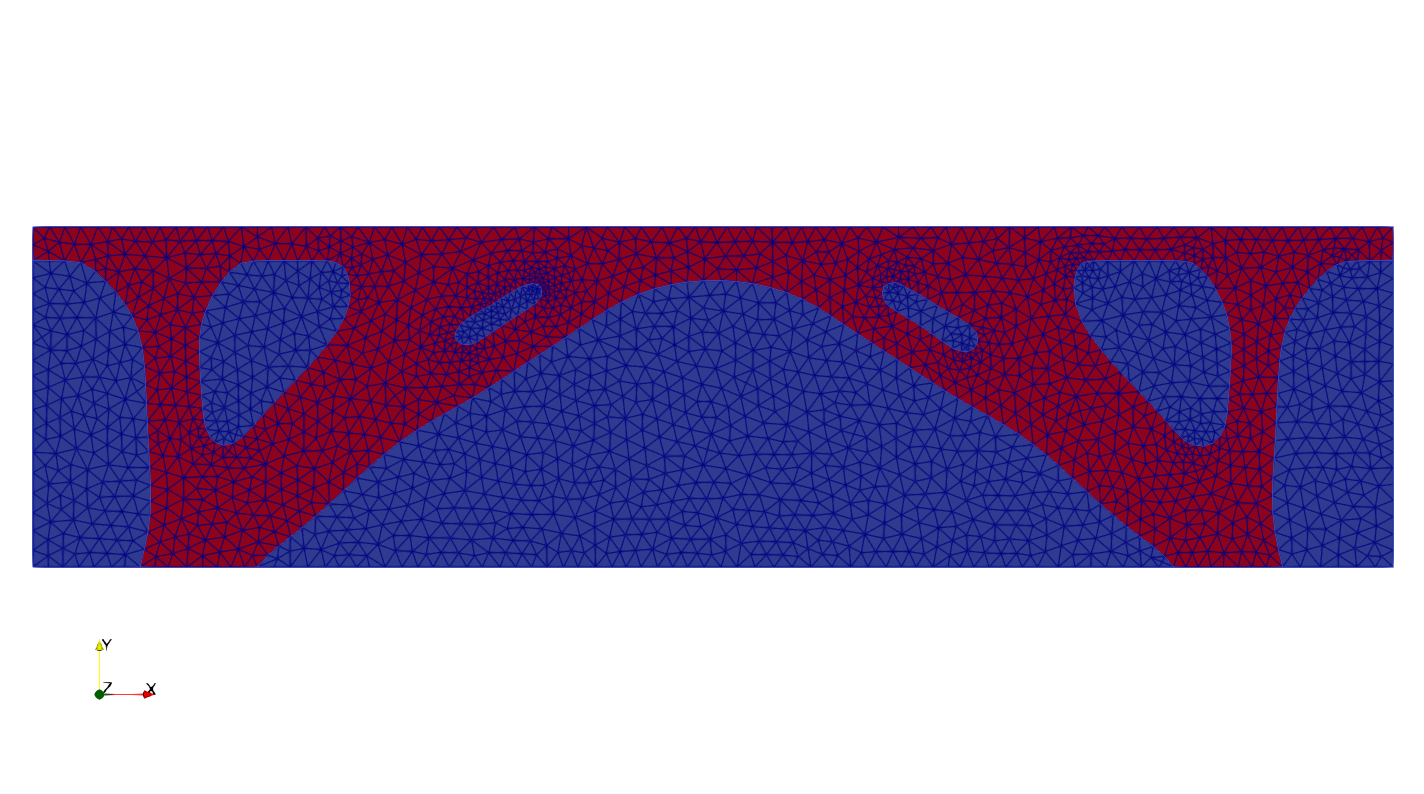
Fig. 14 Optimal shape (in red)#
The demo xml file created is available in the module OpenPisco.Demos() of the OpenPisco Python library 1 .