Tutorials#
This section proposes the following tutorials using the OpenPisco CL and GUI applications
Topology optimization of a cantilever beam using structured level sets
Topology optimization of a cantilever beam using unstructured conformal level sets
Topology optimization of a 2D cantilever beam using conformal level sets
The configuration files created using these tutorials are also available in the module OpenPisco.Demos() of the OpenPisco Python library 1 .
Moreover this section proposes the following tutorial using the OpenPisco Python library
Topology optimization of a cantilever beam using structured level sets#
The goal of this tutorial is to run a topology optimization of a cantilever beam using structured level sets.
Test case#
Consider the following specifications
domain of size \(12\) m \(x 4\) m \(x 3\) m
elastic material with Young modulus equal to \(1\) Pa and Poisson ratio equal to \(0.3\)
beam clamped on the plane \(x = 0\) m and submitted to a vertical load g = \((0, 0, -1000)\) N on the point \((12, 0, 1.5)\)
minimization of the elastic compliance under a volume constraint
Data setting : header#
At first, we start by editing a Liu_Tovar_2014_Cantilever_T4_C1.xml file.
The data file starts with the following header
<data dim="3" debug="False">
Data setting : implicit zones#
Define implicit zones
<Zones>
    <AABox id="10" origin="0. 0.05 0.05" size="12 3.9 2.9" desc="Init" />
    <Gyroid id="100"  desc="Init" scale="0.031831" />
    <Symmetric id="101" z="100" center="12 0 1.5"/>
    <Intersection id="1" z="10 101"/>
    <Plane id="2" point="0.1 0. 0." normal="1. 0. 0." desc="Block"/>
    <Cylinder id="3" center1="12 0 1.47" center2="12 0 1.53" radius="0.03" desc="Force"/>
    <Union id="4" z="2 3"/>
    <Union id="5" z="1 4 "/>
</Zones>
Data setting : grids#
Define the background mesh which is a uniform grid
<Grids>
    <Grid id="1" n="61 41 31" origin="0. 0. 0." length="12 4 3"/>
</Grids>
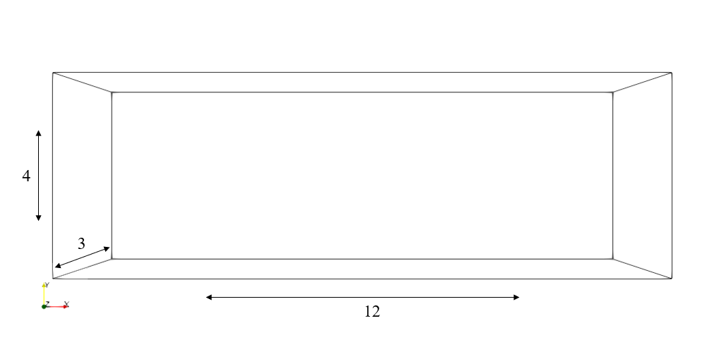
Fig. 2 Grid dimensions#
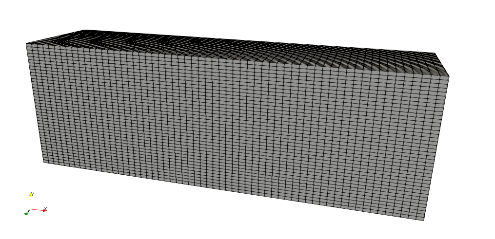
Fig. 3 Structured mesh#
Data setting : levelsets#
Define the level set together with a set of options. By default the level set is structured.
<LevelSets>
    <LevelSet id="1" support="1"/>
</LevelSets>
Data setting : physical problems#
Define the physical problem, which is a linear elastic static FEA problem.
We define one dirichlet condition and one neumann condition.
By default we use linear elements.
The option eVoid=”0.001” means that the density of the Ersatz material equals 0.001.
<PhysicalProblems>
    <Structured id="1" grid="1" type="static_elastic" eVoid="0.001" narrow=".2">
         <Dirichlet zone="2" dofs="0 1 2" val="0.0"/>
         <Neumann   zone="3" dofs="1" val="-1000"/>
    </Structured>
</PhysicalProblems>
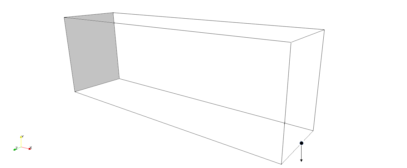
Fig. 4 Boundary conditions for the elastic problem. Clamped zone in light grey (left) and nodal force (right)#
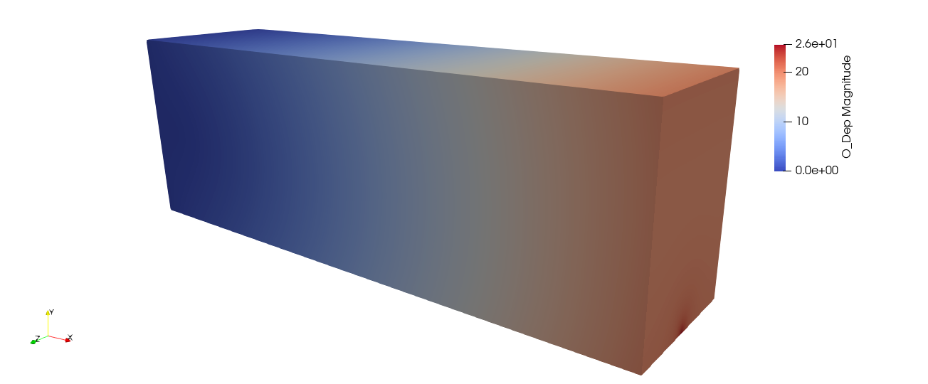
Fig. 5 Displacement field computed on the full design space#
Data setting : outputs#
Define the desired output
<Outputs>
   <Output id="2" name="Liu_Tovar_2014_Cantilever_T4_C1.xdmf"/>
   <Output id="3" name="Liu_Tovar_2014_Cantilever_T4_C1.csv" nTag="NT3" />
   <Output id="1" name="PROXY" outputs="2 3"/>
</Outputs>
Data setting : optimization problems#
Then, we define the optimization problem by entering the objective, the constraints, the initial levelset, the implicit zones, the output and a set of options.
Note that we have to define an upper bound value for the constraint.
Note that, since the objective is a physical criterion, we precise which physical problem should be used with the keyword useProblem=”1”.
<OptimProblems>
    <OptimProblem type="TopoGeneric" id="1"
        OnZone="4"
        useLevelset="1"
        e2="0.001"
        output="1">
      <Objective  type="Compliance"  name="Compliance" useProblem="1" />
      <Constraint type="Volume"     name="Volume"   upperBound="21.6"  desc="0.15*voltotal= 0.15*12*4*3=21.6"/>
   </OptimProblem>
</OptimProblems>
Data setting : optimization algorithms#
Then, we define the optimization algorithm which is linked to the optimization problem
<TopologicalOptimizations>
    <OptimAlgoNullSpace id="1"
    useOptimProblem="1"
    numberOfDesignStepsMax="60"/>
</TopologicalOptimizations>
Actions setting#
Here we declare actions which must be runned. At first, we create a nodal tag labeled “NT3” from the implicit zone “3” of the level set “1”
<Actions>
    <Action type="CreateTagsFromZones" ls="1" nodalTags="3" />
Then, the level set “1” is initialized with the implicit zone “5” and redistanciated to generate a signed distance function
<Action type="InitLevelset" ls="1" zone="5"/>
<Action type="UpdateDistance" ls="1" />
Then, we run the topology optimization
<Action type="RunTopoOp" TopoOp="1"/>
Eventually the optimal shape is exported in stl format
       <Action type="SaveShapeToFile" ls="1" filename="Liu_Tovar_2014_Cantilever_T4_C1.stl"/>
   </Actions>
</data>
Run#
To run the script using the command line application execute in a terminal
OpenPiscoCL Liu_Tovar_2014_Cantilever_T4_C1.xml
To run the script using the GUI application execute in a terminal
OpenPisco Liu_Tovar_2014_Cantilever_T4_C1.xml
Output#
After running the tutorial script the following output files have been created in the working directory
Liu_Tovar_2014_Cantilever_T4_C1.xml.log : run summary
Liu_Tovar_2014_Cantilever_T4_C1.stl : optimal shape in stl format
Liu_Tovar_2014_Cantilever_T4_C1.xdmf : (heavy) file containing the mesh and fields at each iteration in xdmf format
Liu_Tovar_2014_Cantilever_T4_C1.csv : convergence history in csv format

Fig. 6 Visualisation of the optimal design in Paraview#
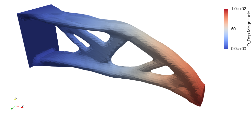
Fig. 7 Visualisation of the displacement field in Paraview#
Topology optimization of a cantilever beam using unstructured conformal level sets#
The goal of this tutorial is to run a topology optimization of a cantilever beam using unstructured conformal level sets.
Test case#
Consider the following specifications
domain of size \(2\) m \(x 0.5\) m \(x 1\) m
elastic material with Young modulus equal to \(210.e9\) Pa and Poisson ratio equal to \(0.3\)
beam clamped on the plane \(x = 0\) m and submitted to a vertical load g = \((0, 0, -10000)\) N on the point \((2, 0.25, 0.5)\)
minimization of the volume under a compliance constraint
Data setting : header#
At first, we start by editing a Cantilever.xml file.
The data file starts with the following header
<data dim="3">
Data setting : implicit zones#
Define implicit zones
<Zones>
    <Plane id="1" point="0.0001 0.25 0.5" normal="1. 0. 0." desc="x0 plane"/>
    <Plane id="2" point="0.05 0.25 0.5" normal="1. 0. 0." desc="dirichlet"/>
    <Plane id="3" point="1. 0.24999 0.5" normal="0. -1. 0." desc="symetry plane"/>
    <Sphere id="4" center="2. 0.25 0.5"  radius="0.0009" desc="nodal force"/>
    <Cylinder id="5" center1="1.9999 0.25 0.5" center2="2.1 0.25 0.5" radius="0.01" desc="force"/>
    <Cylinder id="6" center1="-0.1 0.25 0.5" center2="2.1 0.25 0.5" radius="0.249"/>
    <Union id="7" z="2 4 6" desc="initialization"/>
    <Union id="8" z="2 5" desc="onzone"/>
</Zones>
Data setting : grids#
Define the background mesh which is a uniform grid
<Grids>
    <Grid id="1" n="41 41 41" origin="0. 0. 0." length="2.0 0.25 1.0" ofTetras ="True"/>
</Grids>
Data setting : levelsets#
Define the level set together with a set of options. The option conform=”True” means that the level set is conformal. When the body-fitted option is activated a set of meshing options are defined to drive the remeshing process.
<LevelSets>
    <LevelSet id="1" support="1" conform="True" gradientMethod="gradPhi">
        <MesherInfo hmax=".5" hmin="0.01" iso="0.0" rmc="1e-5"
        nr="True" computeDistanceWith="meshdist"/>
    </LevelSet>
</LevelSets>
Data setting : physical problems#
Define the physical problem, which is a linear elastic static problem.
We define material properties, two dirichlet conditions -clamped part and symetry plane- and one neumann condition.
By default we use linear elements.
<PhysicalProblems>
     <GeneralAster type="static_elastic" id="1" >
               <Material  E="210.e9" Nu="0.3" />
               <Dirichlet eTag="eTag1" dofs="0 1 2" value="0.0"/>
               <Dirichlet eTag="eTag3" dofs="1" value="0.0"/>
               <Force nTag="nTag4" value="0. 0. -10000" />
      </GeneralAster>
 </PhysicalProblems>
Data setting : outputs#
Define the desired output
<Outputs>
   <Output id="2" name="Cantilever.xdmf"/>
   <Output id="3" name="Cantilever.csv" nTag="nTag4" />
   <Output id="1" name="PROXY" outputs="2 3"/>
</Outputs>
Data setting : optimization problems#
Then, we define the optimization problem by entering the objective, the constraints, the initial levelset, the implicit zones, the output and a set of options.
Note that we have to define an upper bound value for the constraint.
Note that, since the objective is a physical criterion, we precise which physical problem should be used with the keyword useProblem=”1”.
<OptimProblems>
    <OptimProblem type="TopoGeneric" id="1"
        OnZone="8"
        useLevelset="1"
    printMeshQualityInfo = "True"
        output="3"
        outputEveryLevelsetUpdate = "False">
      <Objective  type="Volume"  name="Volume"/>
      <Constraint type="Compliance"  name="Compliance" UpperBound="2.5*4.69434000e-01"   useProblem="1" />
   </OptimProblem>
</OptimProblems>
Data setting : optimization algorithms#
Then, we define the optimization algorithm which is linked to the optimization problem
<TopologicalOptimizations>
    <OptimAlgoNullSpace id="1"
       useOptimProblem="1"/>
</TopologicalOptimizations>
Actions setting#
Here we declare actions which must be runned. At first the level set “1” is initialized with the implicit zone “7”
<Actions>
    <Action type="InitLevelset" ls="1" zone="7"/>
Then, we add the bounding box edges and the skin to the initial grid. Moreover, we create tags on elements of dimension 2 starting from the implicit zones “1”,”3”. Tags “eTag1”,”eTag3” are created.
<Action type="AddEdges" ls="1" ar="90+45" />
<Action type="AddSkin" ls="1"/>
<Action type="CreateTagsFromZones" ls="1" elementTags="1 3" dim="2" elemenprefix="eTag"/>
We create a nodal tag “nTag4” from implicit zone “4” for the nodal force and we set it as required to preserve it during the remeshing
<Action type="CreateTagsFromZones" ls="1" nodalTags="4" nodalprefix="nTag"/>
<Action type= "SetAsRequired" ls="1" nTags="nTag4" />
We perform a remeshing to generate a conformal mesh
  <Action type="Remesh" ls="1" hmax=".5" hmin="0.01" iso="0.0" rmc="1e-5"
nr="True" computeDistanceWith="meshdist" />
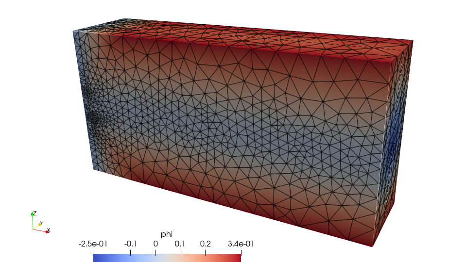
Fig. 8 Background mesh after a first remeshing#
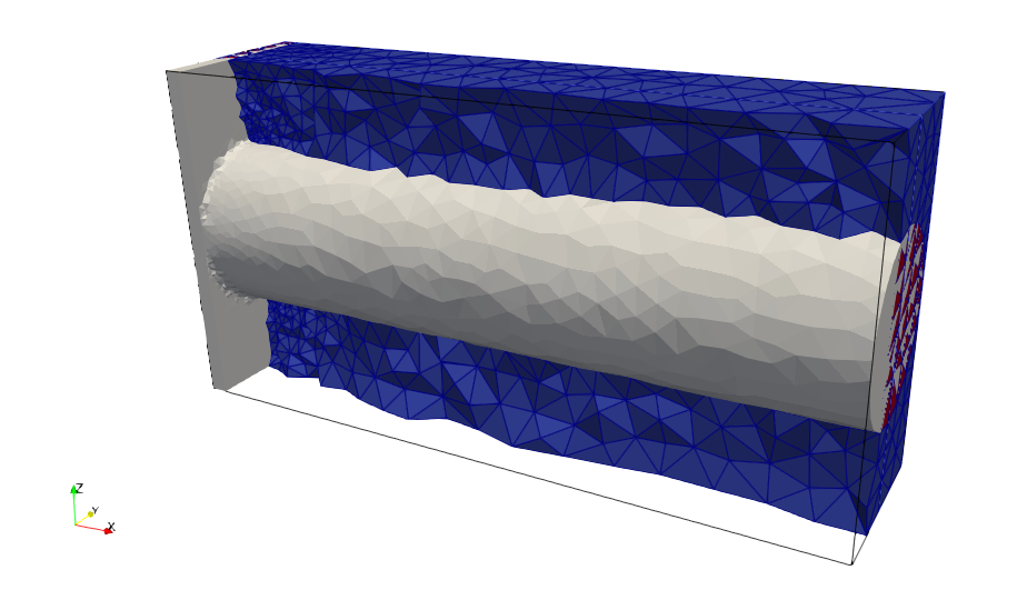
Fig. 9 Cut of the initial body-fitted mesh#
Then, we run the topology optimization
<Action type="RunTopoOp" TopoOp="1"/>
Eventually the optimal shape is exported in stl format
       <Action type="SaveShapeToFile" ls="1" filename="Cantilever.stl"/>
   </Actions>
</data>
Run#
To run the script using the command line application execute in a terminal
OpenPiscoCL Cantilever.xml
To run the script using the GUI application execute in a terminal
OpenPisco Cantilever.xml
Output#
After running the tutorial script the following output files have been created in the working directory
Cantilever.xml.log : run summary
Cantilever.stl : optimal shape in stl format
Cantilever.xdmf : (heavy) file containing the mesh and fields at each iteration in xdmf format
Cantilever.csv : convergence history in csv format
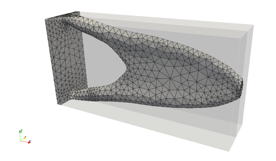
Fig. 10 Visualisation of the optimal design in Paraview#
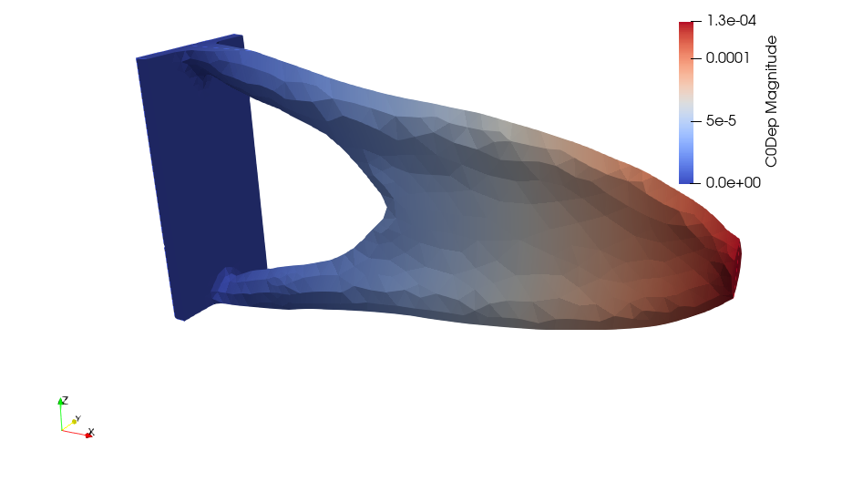
Fig. 11 Visualisation of the displacement field in Paraview#
Topology optimization of a 2D cantilever beam using conformal level sets#
The goal of this tutorial is to run a topology optimization of a bidimensional cantilever beam using unstructured conformal level sets.
Note
For running this tutorial Code_Aster 2 needs to be installed and available from the command line.
Test case#
Consider the following specifications
domain of size \(2\) m \(x 1\) m
elastic material with Young modulus equal to \(210.e9\) Pa and Poisson ratio equal to \(0.3\)
beam clamped on the plane \(x = 0\) m and submitted to a vertical load g = \((0, -10000)\) N on the point \((2, 0.5)\)
minimization of the volume under a compliance constraint
Data setting : header#
We start by editing a Cantilever2D.xml file.
The data file starts with the following header
<data dim="2" >
Data setting : implicit zones#
Define implicit zones
<Zones>
    <Plane id="1" point="0.0001 0.25 0.5" normal="1. 0. 0." desc="x0 plane "/>
    <Plane id="2" point="0.05 0.25 0.5" normal="1. 0. 0." desc="dirichlet"/>
    <Sphere id="4" center="2. 0.5 0.0"  radius="0.0009" desc="nodal force"/>
    <Cylinder id="5" center1="1.9999 0.5 0." center2="2.1 0.5 0." radius="0.01" desc="force"/>
    <Holes id="6" n="6 4 2" r="0.2" boundingMin="0. 0. 0." boundingMax="2.0 1.0 1.0" type="Original" desc="Holes"/>
    <Union id="7" z="2 4 6" desc="initialization"/>
    <Union id="8" z="2 5" desc="onzone" />
</Zones>
Data setting : grids#
Define the background mesh which is a uniform grid
<Grids>
    <Grid id="1" n="61 41" origin="0. 0." length="2.0 1.0" ofSimplex="True"/>
</Grids>
Data setting : levelsets#
Define the level set together with a set of options. The option conform=”True” means that the level set is conformal. A set of meshing options are defined to drive the remeshing process.
<LevelSets>
    <LevelSet id="1" support="1" conform="True" gradientMethod="gradPhi">
          <MesherInfo hmax=".03" hmin="0.008" iso="0.0" rmc="1e-5"
  nr="True" computeDistanceWith="meshdist"/>
    </LevelSet>
</LevelSets>
Data setting : physical problems#
Define the physical problem, which is a linear elastic static problem.
We define material properties, one dirichlet condition and one neumann condition.
By default we use linear elements.
<PhysicalProblems>
    <GeneralAster type="static_elastic" id="1" >
        <Material  E="210.e9" Nu="0.3" />
        <Dirichlet eTag="eTag1" dofs="0 1" value="0.0"/>
        <Force nTag="nTag4" value="0. -1000" />
     </GeneralAster>
</PhysicalProblems>
Data setting : outputs#
Define the desired output
<Outputs>
   <Output id="1" name="Cantilever2DHistory.xdmf" inTempDirectory="True" />
   <Output id="2" name="Cantilever2DHistory.csv" inTempDirectory="True" />
   <Output id="3" name="PROXY" outputs="1 2" />
</Outputs>
Data setting : optimization problems#
Then, we define the optimization problem by entering the objective, the constraints, the initial levelset, the implicit zones, the output and a set of options.
Note that we have to define an upper bound value for the constraint.
Note that, since the constraint is a physical criterion, we precise which physical problem should be used with the keyword useProblem=”1”.
<OptimProblems>
    <OptimProblem type="TopoGeneric" id="1"
        OnZone="8"
        useLevelset="1"
        printMeshQualityInfo = "True"
        output="3"
        outputEveryLevelsetUpdate = "False">
      <Objective  type="Volume"  name="Volume"/>
      <Constraint type="Compliance"  name="Compliance" UpperBound="2*1.90489800e-04" useProblem="1" />
   </OptimProblem>
</OptimProblems>
Data setting : optimization algorithms#
Then, we define the optimization algorithm which is linked to the optimization problem
<TopologicalOptimizations>
    <OptimAlgoNullSpace id="1"
       useOptimProblem="1"/>
</TopologicalOptimizations>
Actions setting#
Here we declare actions which must be runned. At first the level set “1” is initialized with the implicit zone “7”
<Actions>
    <Action type="InitLevelset" ls="1" zone="7"/>
We create a nodal tag “nTag4” from implicit zone “4” for the nodal force and we set it as required to preserve it during the remeshing
<Action type="CreateTagsFromZones" ls="1" nodalTags="4" nodalprefix="nTag"/>
<Action type= "SetAsRequired" ls="1" nTags="nTag4" />
We perform a remeshing to generate a conformal mesh
  <Action type="Remesh" ls="1" hmax=".03" hmin="0.008" iso="0.0" rmc="1e-5"
nr="False" computeDistanceWith="meshdist" />
We create an element tag to support the Dirichlet boundary condition
<Action type="CreateTagsFromZones" ls="1" elementTags="1" dim="1" elemenprefix="eTag"/>
Then, we run the topology optimization
<Action type="RunTopoOp" TopoOp="1"/>
Eventually mesh quality indicators are printed
       <Action type="LsQualityInfo" ls="1" />
   </Actions>
</data>
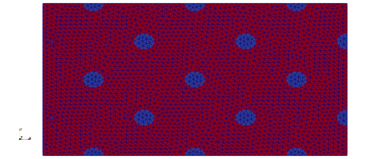
Fig. 12 Visualisation of the initial material distribution in Paraview#
Run#
To run the script using the command line application execute in a terminal
OpenPiscoCL Cantilever2D.xml
To run the script using the GUI application execute in a terminal
OpenPisco Cantilever2D.xml
Output#
After running the tutorial script the following output files have been created in the working directory
Cantilever2D.xml.log : run summary
Cantilever2DHistory.xdmf : (heavy) file containing the mesh and fields at each iteration in xdmf format
Cantilever2DHistory.csv : convergence history in csv format
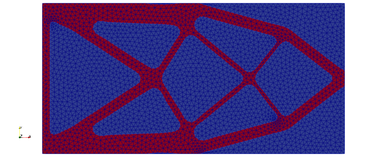
Fig. 13 Visualisation of the optimal design in Paraview#
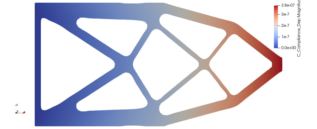
Fig. 14 Visualisation of the displacement field in Paraview#
Conformal remeshing using implicit geometries and mmg3d#
The goal of this tutorial is to create body-fitted meshes using implicit geometries and the remeshing software mmg3d. In order to do so, we start by editing a HoneyComb.xml file
<data dim="3">
We define the honeycomb implicit geometry
<Zones>
    <Honeycomb id="1" lx="0.3" w="0.05" desc="honeycomb implicit zone "/>
</Zones>
We define the initial grid and the conformal level set
<Grids>
    <Grid id="1" n="201 51 101" origin="0. 0. 0." length="2.0 0.5 1.0" ofTetras ="True"/>
</Grids>
<LevelSets>
    <LevelSet id="1" support="1" conform="True"></LevelSet>
</LevelSets>
We define the actions to run
<Actions>
    <Action type="InitLevelset" ls="1" zone="1"/>
    <Action type="AddEdges" ls="1" ar="90+45" />
    <Action type="Remesh" ls="1" hmax=".4" hmin="0.004" hausd="0.004" iso="0.0" rmc="1e-5"" nr="True"/>
    <Action type="WriteToFile" ls="1" filename="{INPUTFILE}.xdmf" />
</Actions>
We close the xml file
</data>
Run#
To run the script using the command line application execute in a terminal
OpenPiscoCL HoneyComb.xml
To run the script using the GUI application execute in a terminal
OpenPisco HoneyComb.xml
Output#
After running the following output files have been created in the working directory
HoneyComb.xml.log : run summary
HoneyComb.xdmf : file containing the body-fitted mesh created
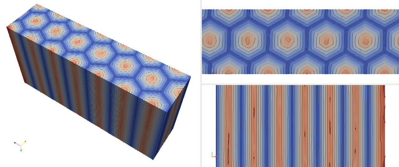
Fig. 15 Honeycomb implicit geometry#
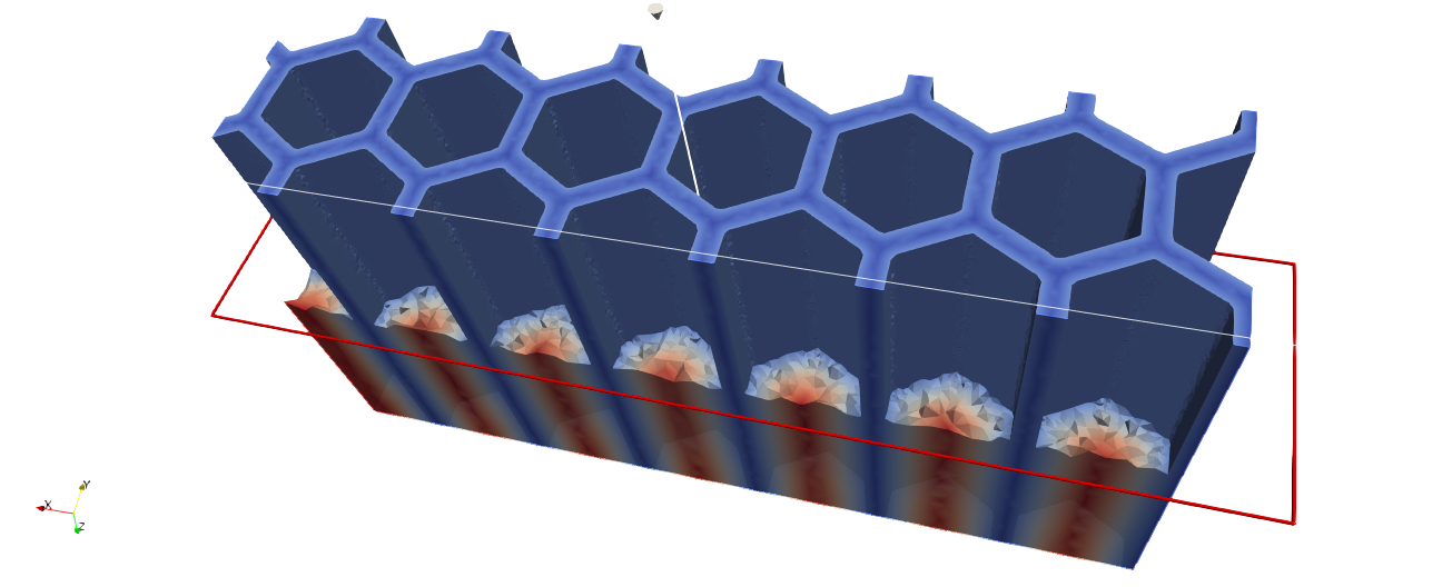
Fig. 16 Honeycomb-shaped body-fitted mesh#
Overhanged surfaces detection for additive manufacturing#
The goal of this tutorial is to detect and export overhanged surfaces for additive manufacturing. At first we start by editing an OverHangDetection.xml file, reading the input mesh model and instanciating a level set
<data dim="3" debug="False" >

    <Grids>
        <Mesh id="1" filename="{PISCO_TEST_DATA}TubeMesh.msh" />
    </Grids>

    <LevelSets>
        <LevelSet id="1" support="1" conform="True">
        </LevelSet>
    </LevelSets>
We detect the overhanged surfaces for an input angle of 45 degrees in the direction \((0, 0, 1)\). The keyword surfaceTags is optional and allows to run the overhang detection on specific mesh tags. Read the docstring of OpenPisco.Actions.AdditiveManufacturingActions.OverHangDetectionAction for the complete list of options. The routine computes the triangle normals to check if the overhang condition is fulfilled. Doing so a tag named”overhangSurface” is filled with the overhanged triangles and added to the mesh tags.
<Actions>
    <Action type="OverHangDetection" ls="1" angleDetection="45" surfaceTags="OutsideTube InsideTube" direction="0 0 1"/>
Eventually we export the overhanged surfaces and close the input file
       <Action type="WriteSurfaceToStl" eTag="overhangSurface" ls="1"/>
   </Actions>
</data>
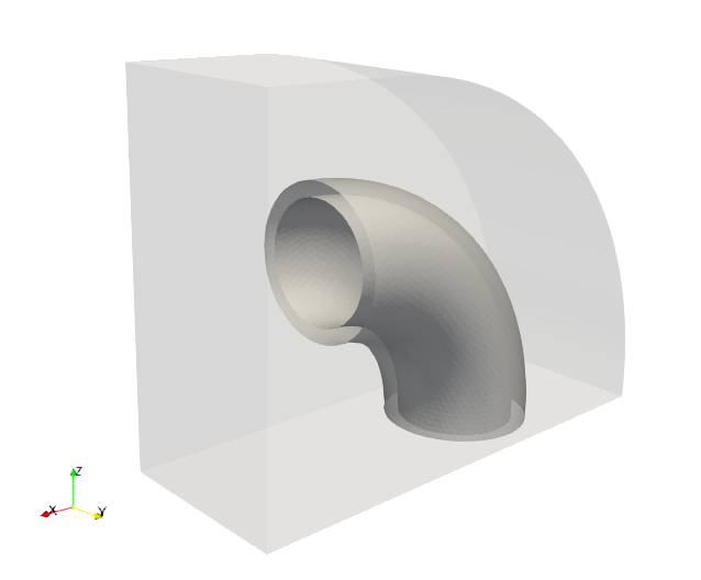
Fig. 17 Input model with selected mesh tags “OutsideTube” and “InsideTube”#

Fig. 18 Detected overhanged surfaces#
Topology optimization of a bridge using conformal level sets#
The goal of this tutorial is to run a topology optimization using solely the OpenPisco Python library.
Test case#
Consider the following specifications
domain of size \(8\) m \(x 2\) m
elastic material with Young modulus equal to \(1\) Pa and Poisson ratio equal to \(0.3\)
beam clamped on two regions on the plane \(y=0\) and submitted to a vertical load g = \((0, -0.002)\) N on the plane \(y=2\)
minimization of the compliance under a volume constraint
Data setting : imports#
We start by editing a Bridge.py file and importing all the needed modules
import numpy as np

from Muscat.MeshTools.MeshCreationTools import CreateSquare
from Muscat.ImplicitGeometry.ImplicitGeometryObjects import CreateImplicitGeometryPlane, ImplicitGeometryHoles,CreateImplicitGeometryAnalytical
from Muscat.ImplicitGeometry.ImplicitGeometryOperators import ImplicitGeometryUnion, ImplicitGeometryIntersection
from Muscat.MeshContainers.Filters.FilterObjects import ElementFilter
from Muscat.IO.XdmfWriter import XdmfWriter

from OpenPisco.Unstructured.Levelset import LevelSet
from OpenPisco.PhysicalSolvers.UnstructuredFEAGenericSolver import CreateUnstructuredFEAGenericProblem
from OpenPisco.Optim.Problems.OptimProblemTopoGeneric import OptimProblemTopoGeneric
from OpenPisco.Optim.Criteria.GeoCriteria import TopoCriteriaVolume
from OpenPisco.Optim.Criteria.PhyCriteria import TopoCriteriaCompliance
from OpenPisco.Optim.Algorithms.OptimAlgoNullSpace import OptimAlgoNullSpace
Data setting : implicit zones#
Define implicit zones
IGHoles = ImplicitGeometryHoles()
IGHoles.r = 0.2
IGHoles.n = np.array([6., 4., 2.])
IGHoles.type = "Original"

IGGeometryPlane = CreateImplicitGeometryPlane({"point": [0, 1.8, 0], "normal": [0, -1, 0]})

IGAnalytical1 = CreateImplicitGeometryAnalytical({"expr": "x-1 "})
IGAnalytical2 = CreateImplicitGeometryAnalytical({"expr": "x-7 "})
IGAnalytical2.insideOut = True
IGAnalytical3 = CreateImplicitGeometryAnalytical({"expr": "y-0.01 "})

IGUnion = ImplicitGeometryUnion([IGAnalytical1,IGAnalytical2])
IGIntersection = ImplicitGeometryIntersection([IGUnion,IGAnalytical3])
Data setting : grids#
Define the initial background mesh which is a uniform grid
dimensions = np.array([25,20])
length = np.array([8,2])
mesh= CreateSquare(dimensions=dimensions, spacing=length/(dimensions-1), origin=[0,0], ofTriangles=True)
Add ridges and corners to the mesh
for _,data,_ in ElementFilter(dimensionality=1)(mesh):
    data.tags.CreateTag("Ridges",False).SetIds(np.arange(data.GetNumberOfElements()))

mesh.nodesTags.CreateTag("Corners",errorIfAlreadyCreated=False).Merge(other=mesh.nodesTags[ "x0y0"])
mesh.nodesTags.CreateTag("Corners",errorIfAlreadyCreated=False).Merge(other=mesh.nodesTags[ "x1y0"])
mesh.nodesTags.CreateTag("Corners",errorIfAlreadyCreated=False).Merge(other=mesh.nodesTags[ "x0y1" ])
mesh.nodesTags.CreateTag("Corners",errorIfAlreadyCreated=False).Merge(other=mesh.nodesTags[  "x1y1" ])
Create mesh tag on elements of dimensionality equal to 1 for Dirichlet boundary condition
ff = ElementFilter()
ff.SetZones([IGIntersection])
ff.SetDimensionality(1)
for _,data,ids in ff(mesh):
    data.tags.CreateTag("Dirichlet").SetIds(ids)
Print the mesh
print(mesh)
Data setting : levelsets#
Define the level set together with a set of options. A set of meshing options are defined to drive the remeshing process.
levelset = LevelSet(support=mesh)
levelset.conform = True
levelset.MesherInfo = {"gradientMethod":"gradPhi","hmax":0.1,"hmin":0.01,"rmc":1e-5,"hausd":0.01,"nr":True,"iso":0.0}

IGHoles.SetSupport(levelset.support)
levelset.phi = IGHoles(levelset.support)
Data setting : physical problems#
Define the physical problem, which is a linear elastic static problem.
We define material properties, one dirichlet condition and one neumann condition.
The linear solver used is Mumps 3.
material = ('Material', {'young': '1', 'poisson': '0.3'})
dirichlet = ('Dirichlet', {'eTag': 'Dirichlet', 'dofs': '0 1', 'value': '0'})
load = ('Force', {'eTag': 'Y1', 'dir': '0 1', 'value': '-0.002'})
data = {'type': 'static_elastic', 'p': '1','dimensionality':'2',"linearSolverName":"Mumps",'children':[material,dirichlet,load]}
physicalSolver = CreateUnstructuredFEAGenericProblem(data)
Data setting : optimization problems#
Then, we define the optimization problem by entering the objective, the constraints, the initial levelset, the fixed implicit zone and a set of options.
Note that we have to define an upper bound value for the constraint.
res = OptimProblemTopoGeneric()
volCrit = TopoCriteriaVolume()
comCrit = TopoCriteriaCompliance()
res.SetObjectiveCriterion(comCrit)
res.AddInequalityConstraint(volCrit)
volCrit.SetUpperBound(0.4*1.55651243e+01)
comCrit.problem = physicalSolver
res.point = levelset
res.ResetState()
res.OnZone = IGGeometryPlane
Data setting : outputs#
Define the writer to get the output files
writer = XdmfWriter('Bridge2DHistory.xmf')
print("Opening file :"+writer.fileName)
writer.SetTemporal()
writer.SetBinary()
writer.SetXmlSizeLimit(0)
writer.Open()
res.writer = writer
Data setting : optimization algorithms#
Then, we define the optimization algorithm which is linked to the optimization problem
OA = OptimAlgoNullSpace()
OA.ResetState()
OA.alphaC = 0.5
OA.tol_merit =  0.001
OA.optimProblem =res
Run#
Run the topology optimization
OA.Start()
To run the script execute in a terminal
python Bridge.py
Output#
After running the tutorial script the following output files have been created in the working directory
Bridge.xml.log : run summary
BridgeHistory.xmf : (heavy) file containing the mesh and fields at each iteration in xmf format
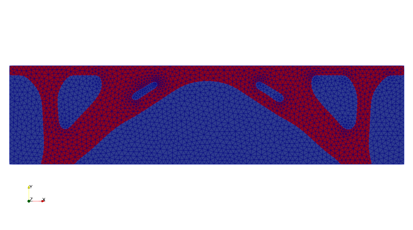
Fig. 19 Optimal shape (in red)#